3 advanced Google Sheets functions: IFERROR, IF & DATEDIF

If you work with numbers or any kind of data sets, you know how much time, energy, and frustration spreadsheet functions can save you. Bye bye manual, tedious calculations! Using the right function for a calculation is a game changer.

Continuing in our efforts to help you become a Google Sheets wiz, we’re sharing three more advanced Google Sheets functions you can start using today. We’ll discuss and show examples of:

How to handle errors
Working with the IF statements
Working with dates.

We promise, these functions will make your life easier when it comes to dealing with lots of data in a spreadsheet.

1. How to use the IFERROR function to handle errors in Google Sheets

If you’ve been using spreadsheets for any serious amount of time, you’re bound to have encountered cell errors. These errors occur when you try to do a calculation that the spreadsheet can’t handle, and they can be a real pain.

Sometimes it’s just an issue of style. Rather than displaying an ugly error in your data, you’d rather show a blank or a zero. The bigger problem though is when errors prevent subsequent calculations from working elsewhere in your spreadsheet.

Some errors like #DIV/0!, which happen if you try and divide a number by zero, aren’t easily avoidable. Others like #VALUE!, which occur when you try and perform a mathematical operation like multiplication or division using a cell that contains text, can often be circumvented by cleaning up your data first. However, that’s not always possible.

The solution is to use Google Sheets’ IFERROR() function. It checks a value for errors, and if it encounters one it replaces the value with whatever you specify. If it doesn’t detect an error it just returns the original value.

Here’s an example:

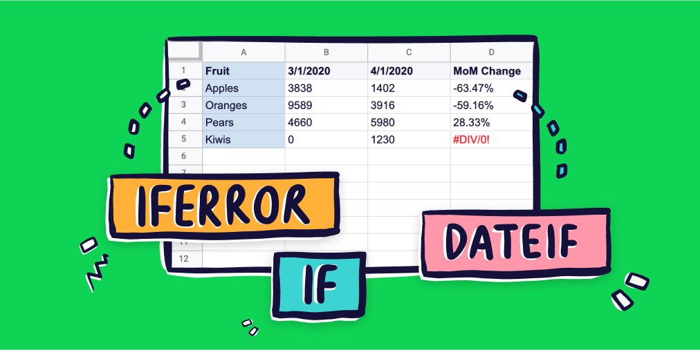
Fruit	3/1/2020	4/1/2020	MoM Change
Apples	3838	1402	-63.47%
Oranges	9589	3916	-59.16%
Pears	4660	5980	28.33%
Kiwis	0	1230	#DIV/0!

The ‘MoM Change’ column for Kiwis contains the calculation: (C5/B5)- 1. This returns #DIV/0 because no Kiwis were sold in March. We can replace #DIV/0 with ‘N/A’ (or anything else of our choosing) by updating the formula to =IFERROR((C5/B5 - 1),“N/A”).

IFERROR checks the value for (C5/B5) -1, sees that the result is an error because you’re trying to divide by zero, and so returns the text “N/A”.

2. How to use Google Sheets’ IF function

IFERROR is just the tip of the iceberg when it comes to what’s possible with Google Sheets’ Logical Functions. There’s also AND, FALSE, NOT,
OR, and TRUE functions. IF is the most useful of these.

IF evaluates a logical expression and returns a different value depending on whether it’s TRUE or FALSE.

The possibilities of this are endless, but here are some examples of what you can achieve.

IF statement to determine pass or fail

Imagine you have a series of test results and you want to classify them as pass or fail depending on whether they score higher than 80%. All you need to do is write:

=IF(B1>0.8, “Pass”, “Fail”)

Name	Score	Pass / Fail
Tom	90%	Pass
Ben	59%	Fail
Sally	79%	Fail
Freya	91%	Pass
Jake	75%	Fail
Katy	81%	Pass

Here’s a list of the various conditions you can test:

A > B A is greater than B
A < B A is less than B
A >= B A is greater than or equal to B
A <= B A is less than or equal to B
A = B A equals B
A <> B A does not equal B

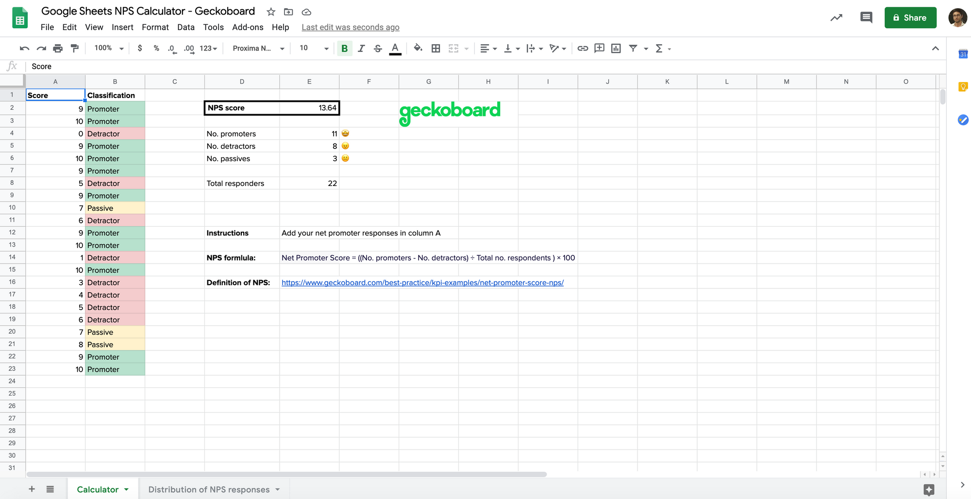
Calculating NPS Net Promoter Score (NPS) in Google Sheets using the IF statement

In a slightly more complex example, imagine we want to use Google Sheets to calculate a Net Promoter Score (NPS).

NPS is a method to measure customer loyalty and product/service virality. Customers are asked to score from 0 to 10 how likely they would be to recommend your company/product/service to a friend or colleague. The score is then worked out by subtracting the number of detractors from promoters and dividing that by the total number of respondents. Detractors are classified as anyone who gives you a rating of 6 or less and promoters as anyone with a score of 9 or 10.

To do this in your spreadsheet, you need to convert the scores to the right categories like we did with our pass or fail example. However, because there are three categories (Detractor, Promoter and Passive) instead of just two, it’s not possible with a single IF statement.

You can solve this by nesting a second IF statement inside the first. The first statement checks if the number is 6 or less. If it’s true it returns “Detractor”, if it’s false then it performs the second check and based on whether that’s true or false returns “Promoter” or “Passive”.

=if(B2<=6,"Detractor",if(B2>=9,"Promoter","Passive"))

But a better solution is to use the IFS function.

=ifs(B1 <=6, "Detractor", A2 >=9, "Promoter",TRUE, "Passive")

IFS allows you to test multiple conditions and it returns the first answer that is true. Here we’ve used TRUE at the end as a trick to mop up the Passive scores, but you could just have easily written formula as:

=ifs(B1 <=6, "Detractor", B1 < 9, "Passive", B1 >=9, "Promoter")

There are always multiple ways to skin a cat when it comes to Google Sheets, and you could also use the SWITCH function.

To actually calculate your NPS score you can then use COUNTIF to count the number of promoters and detractors. COUNTA is a way to count the total number of responses. It counts any cell with a value in it. Just remember it also counts heading rows, so if your spreadsheet contains a header start it at the second row.

=(countif(C:C,"Promoter") - countif(C:C,"Detractor"))/ counta(C2:C)

Here’s a Google Sheet template we’ve put together for calculating NPS:
Copy it here

How to group countries into regions using IF and OR

Imagine you want to label certain countries as being part of a region.

Here’s an example using an OR statement within the IF to assign values that are “USA” or “Canada” as “Domestic” and everything else as “Rest of World”.

=if(OR(A2="USA",A2="Canada"),"Domestic", "Rest of World")

If you wanted to group by continent you could use multiple OR statements inside an IFS, but this would get complicated quicker. A simpler approach would be to add a table of countries and their continents to your spreadsheet and use VLOOKUP.

3. How to use Google Sheets’ DATEDIF function

Calculating the number of days between two dates can be a pain. Maybe you need to know the number of days between now and a launch, or a daily rate of change.

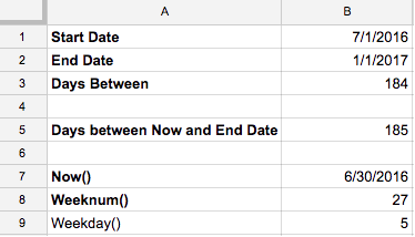
The DATEDIF() function makes life much simpler. Provide it with a Start Date, End Date and Unit (e.g Y for year, M for month, D for day) and it will tell you the quantity (of years, months, or days) between them.

Combining with the NOW() function which returns the current date and time, it’s easy to show the number of days between now and a specified date in the future:
=datedif(now(),B2,"d")

These two functions are particularly helpful for creating a countdown dashboard.

Similar to NOW() there’s also TODAY() which returns just the date rather than date and time.
Some other useful date functions include:

WEEKNUM() - this returns what week of the year it is when provided with a date
WEEKDAY() - this returns what day of the week it is as a number

Google Sheets DATEDIF Function

Now your data can function (pun intended) at new heights with your newfound Google Sheets expertise. Life just got a little easier.

Learn more about Google Sheets Functions

Want to take your spreadsheet game even further? Now that you’ve imported data from various sources into your Google Sheets spreadsheets, you can easily visualize and share this information using a dashboard.

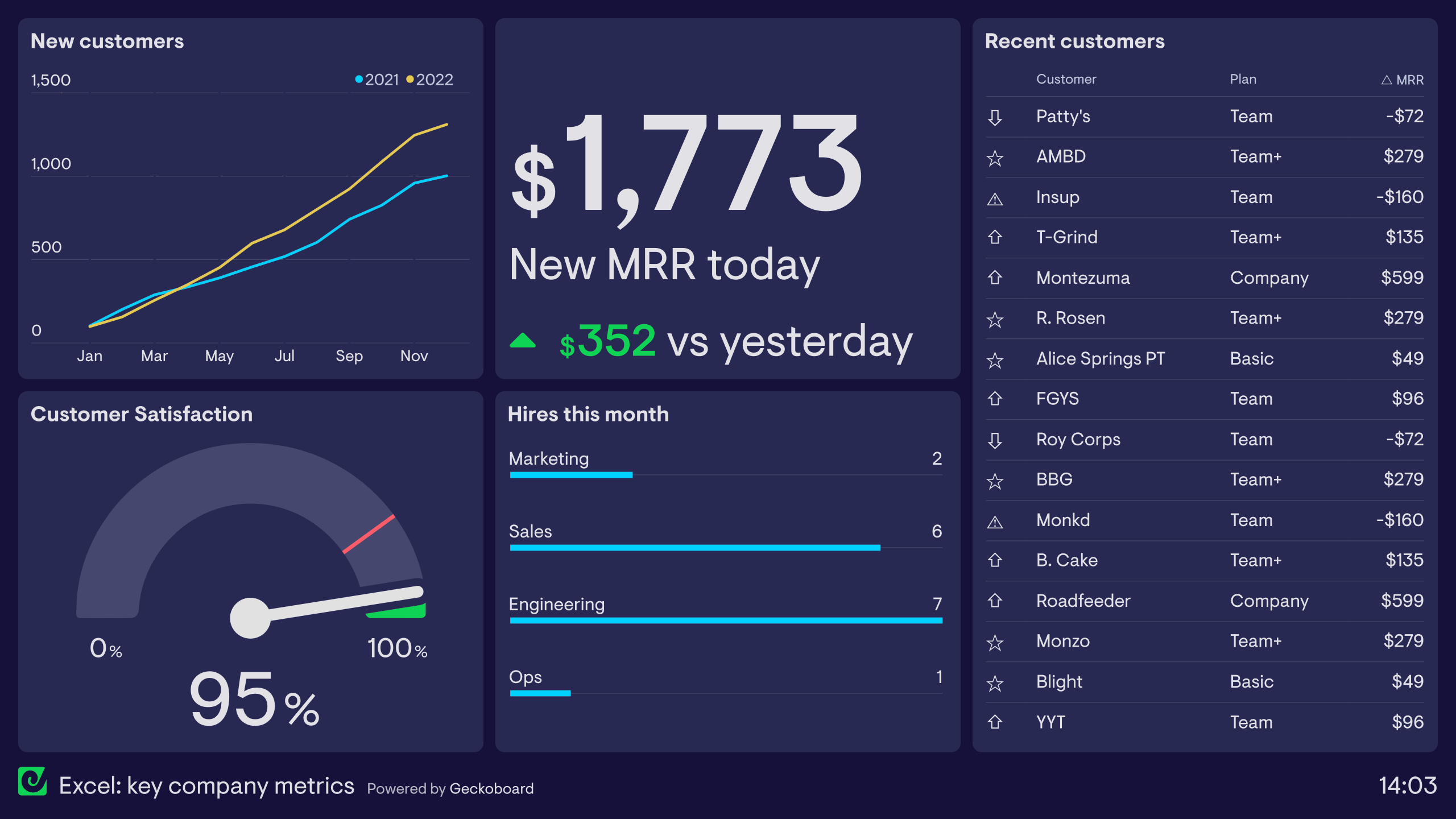
excel-example-dashboard-geckoboard

Learn more about this spreadsheet dashboard example here.

The example above contains a variety of visualizations, which can be powered either by Google Sheets or an Excel spreadsheet, which updates automatically to show up-to-the-minute data.

Here's how it works

Create your spreadsheet in Google Sheets (importing data from via the steps mentioned earlier in this post)
Sign up for a free Geckoboard account
Select ‘Add dashboard’, then ‘Add widget’
Pick the ‘Spreadsheet’ integration from the list of data sources.
Select your data and choose a visualization
Build out your dashboard by adding more visualizations

Watch this in action in the video below!

Originally published on 5th July 2016, updated on 6th October 2022

3 advanced Google Sheets functions that will make your life easier

1. How to use the IFERROR function to handle errors in Google Sheets