Google Sheets is an incredibly versatile and powerful tool that excels (pun intended) at organizing and calculating data in a spreadsheet format. Being cloud-based, it offers many possibilities for collaborating, automating data collection, and even for pulling data in from third-party APIs, using a handful of simple but powerful functions.
Whether you’re just getting up to speed with Google Sheets, or looking to up your spreadsheet game more generally, here are some of our six favourite Google Sheets functions to help you get the most out of your spreadsheets.
Overview
Click a Google Sheets function below to read about it.
- How to join text in Google Sheets
- How to return the first or last value in a Google Sheet using the INDEX function
- How to import data into Google Sheets using IMPORT functions
- How to use VLOOKUP & HLOOKUP to join data in Google Sheets
- How to COUNT and SUM values
- How to group data in Google Sheets using pivot tables

1. How to join text in Google Sheets
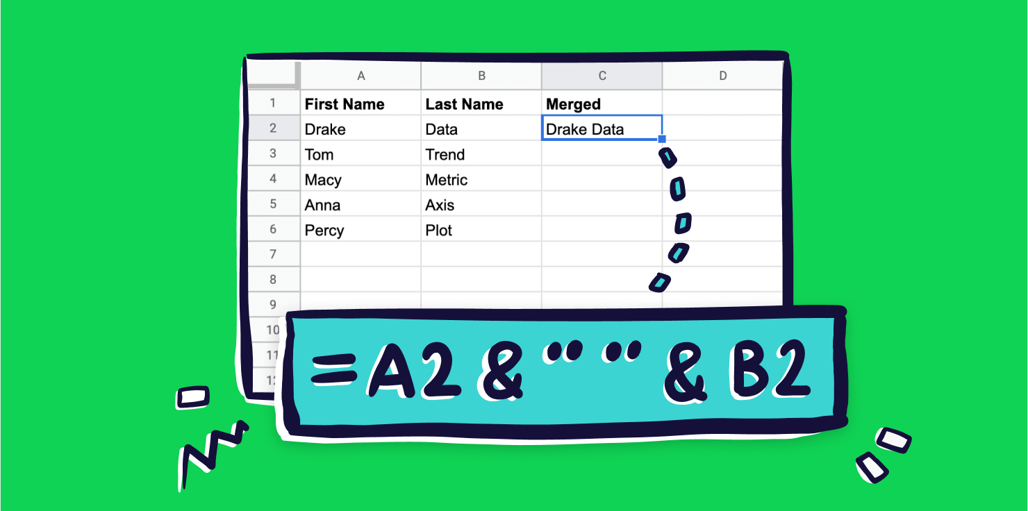
Sometimes it can be handy to use the cells in your spreadsheet to construct a piece of text - perhaps to summarise some key values, or even generate some html.
By typing & you can concatenate (join) the contents of a cell with others or, using quotes, any other text you wish to insert.
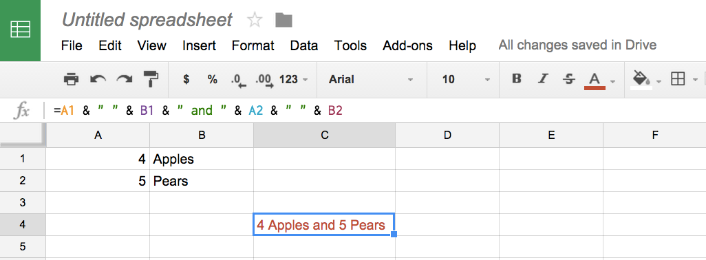
In the example below we’ll use the following formula:
=A1 & " " & B1 & " and " & A2 & " " & B2
to produce the following text “4 Apples and 5 Pears”
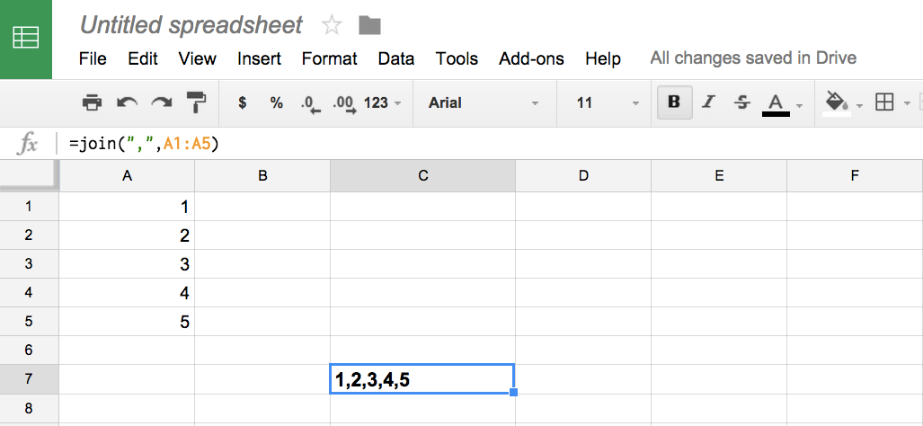
If you’d like to combine lots of values in a Google Sheet, the JOIN function is also useful. You specify what character you’d like to add between the values, and the cell values you’d like to join.
In the example below the formula:
=join(",",A1:A5)
Will join the values to produce:
1,2,3,4,5
2. How to return the first or last value in a Google Sheet using the INDEX function
Spreadsheets are much easier to work with when you have a fixed data set. However, if you’re adding new data at regular intervals, perhaps a new row every week, there’s often some maintenance required to keep your functions working.
For example, imagine you always want to calculate the change between the bottom cell in your spreadsheet with the previous value. This is surprisingly difficult to do if you want the result to be calculated in a fixed cell every time. There’s no LAST() function.
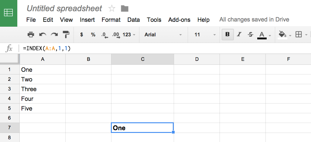
However, there is a solution; the INDEX function. In Google Sheets, the formula INDEX() allows you to return the value of a cell by specifying which row and column to look at in the specified array.
=INDEX(A:A,1,1) for example will always return the first cell in column A.
Combining INDEX() with COUNTA() you can also create a formula that will always get the last value in a column.
=INDEX(A:A,COUNTA(A:A),1)
3. How to import data into Google Sheets using IMPORT functions
One of Google Sheets’ more unexpected features are its IMPORT functions.
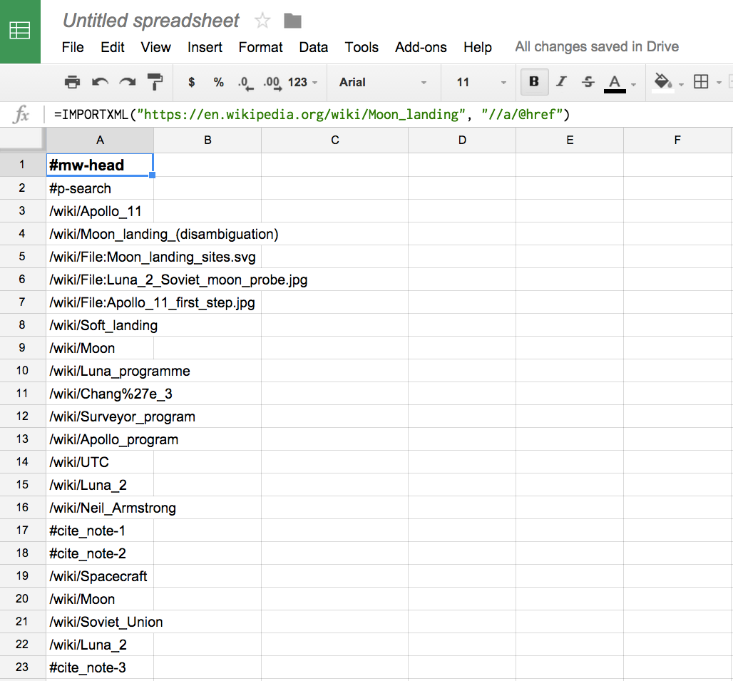
These allow it to fetch data into your spreadsheet from a variety of sources, including XML, HTML, RSS and CSV - perfect for importing lists of blog posts, tweaks, product inventories or data from another service. For example, you can import a list of links from a specified URL with...
=IMPORTXML("https://en.wikipedia.org/wiki/Moon_landing", "//a/@href")
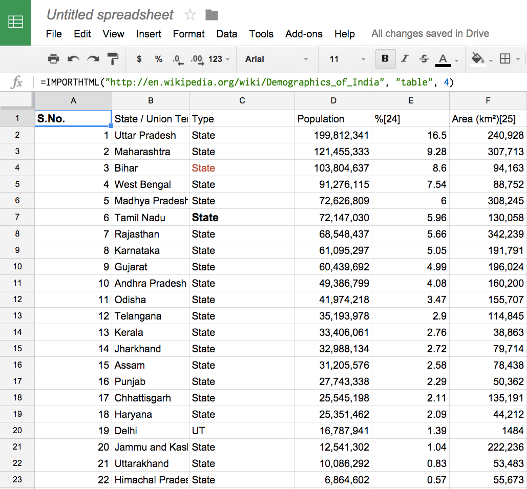
Import the contents of a list or table from a specified URL using:
=IMPORTHTML("http://en.wikipedia.org/wiki/Demographics_of_India", "table", 4)
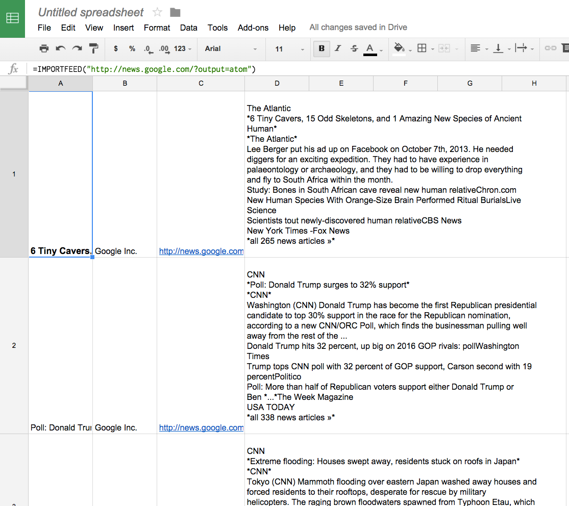
Import an RSS or Atom feed using:
=IMPORTFEED("http://news.google.com/?output=atom")
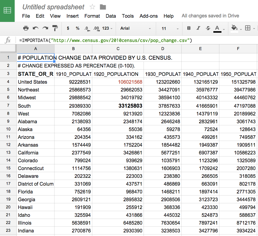
Import the contents of a CSV file from a specified URL using:
=IMPORTDATA(https://www2.census.gov/programs-surveys/bds/tables/time-series/bds2020.csv)
Coupled with Google Sheet’s’ scripting and automation features, IMPORT functions become a very powerful tool for scraping and structuring data from public sources. Use responsibly!
For more ways to get your data into Google Sheets check out our 4 ways to automagically import live data into spreadsheets post.
4. How to use VLOOKUP & HLOOKUP to join data in Google Sheets
Google Sheets’ LOOKUP functions are best explained with an example. In a nutshell, they let you search for a match for a specific word (or other ID) and then read a value from a corresponding row or column. This can be really handy if you have different sets of data for the same objects in your spreadsheet, for example, several rows of data about an individual product, person, or project.
In the example below, imagine you want to track the change in numbers of Apples, Oranges and Pears between January and February. The order of the fruits, and what fruits are available change each month, so a simple fixed cell subtraction won’t work.
Instead, with VLOOKUP() you can tell Google Sheets to look vertically through a set of data until it finds a match for the word you’re searching for and then read horizontally to find the corresponding value in an adjacent column. VLOOKUP stands for Vertical Lookup because it looks vertically for the word then horizontally for the value while HLOOKUP stands for Horizontal Lookup because it looks horizontally for the word and then vertically for the value.
Let’s start with a VLookup using the below table and using the formula:
=VLOOKUP(F2,$A$2:$B$6,2,false)
Within the brackets, “F2” is telling the VLOOKUP to find the value “Apples”, which you find in cell F2. Because it’s a VLOOKUP, the section of the formula “$A$2:$B$6” is telling Google sheets to look vertically in the January data (cells A2 to B6) for the value Apple. The “2” in the formula is telling the VLOOKUP that, when it finds “Apple”, it should look in the second column for the value. The “false” is telling it that, if it doesn’t find the value, it shouldn’t do anything. Ultimately, this formula is looking for Apples in the January data set and then returns the value, 1003, in the second column.
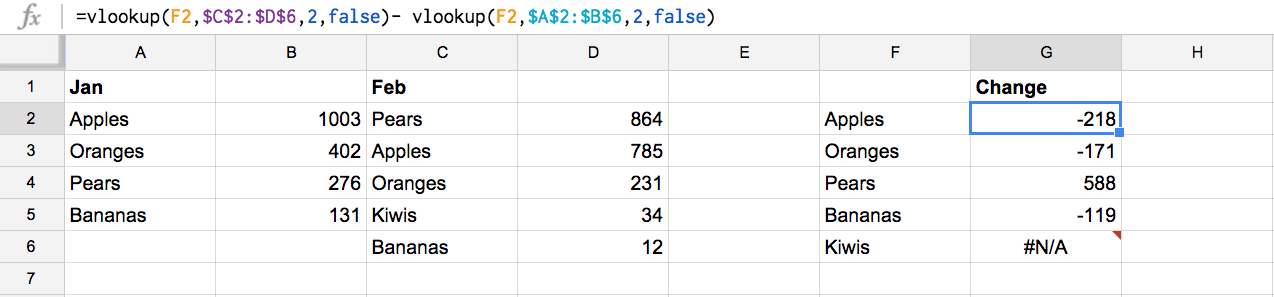
To calculate the change, the lookup for February needs to be subtracted from the lookup for January, so we add to the formula as below:
=VLOOKUP(F2,$C$2:$D$6,2,false)-VLOOKUP(F2,$A$2:$B$6,2,false)
The second part of this formula is the same as above, but now we’re adding the February data and telling Google Sheets to subtract the January data from it. So, by taking the same formula as January and changing “$A$2:$B$6” for “$C$2:$D$6”, we’re telling Google Sheets to do the same VLOOKUP, but for February. This is saying: Look at how many apples were purchased in February (785) and subtract how many apples were purchased in January (1003), returning a value of -218.
Similarly, HLOOKUP() performs the same function but reads across and then looks down once it has a match. More information on both functions can be found here:
There are some limitations with VLOOKUP and HLOOKUP. If you’re feeling adventurous check out this article on how to combine MATCH with INDEX for even more powerful lookups in Google Sheets.
5. How to count and sum values if they contain a certain value in Google Sheets
SUMIF() and COUNTIF() formulas are a bit easier to get your head around than LOOKUPS. They do what they say - they allow you to sum or count values if they match some criteria.
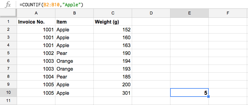
In the example below, you can count the number of Apples sold with a formula like:
=COUNTIF(B2:B10,"Apple")
We’re saying: Count the number of instances of the word “Apple” in cells B2 to B10.
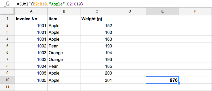
You can also sum the total weight of Apples sold using the SUMIF function.
=SUMIF(B2:B10,"Apple",C2:C10)
We’re telling Google Sheets to look for mentions of the word “Apple” in column B and calculate the total values of the corresponding cells in column C.
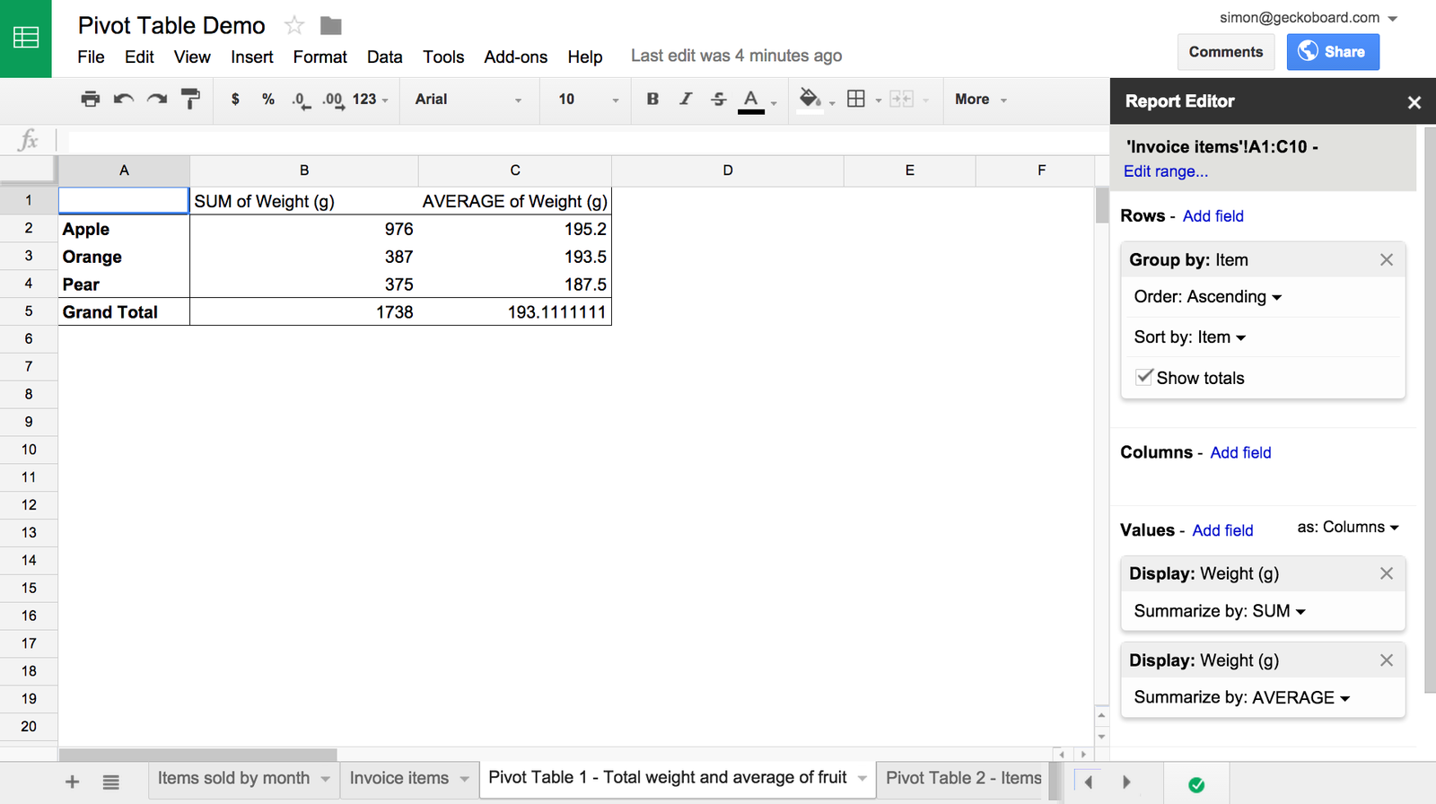
6. How to group data in Google Sheets using pivot tables
Pivot tables are one of the most powerful features in any spreadsheet application and Google Sheets’ implementation is particularly good. You can open a pivot table by selecting the data you want to use and then clicking Data >> Pivot Table.
Pivot table reports make it really easy to bucket, filter, sort and summarise your data using an editor in Google Sheets, rather than using a complex formula. As an example, with pivot tables you can do the same thing we just did with COUNTIF and SUMIF for all fruit without having to use any formula. Beyond counting and summing, it’s also easy to calculate other values such as averages and variances as you can see in the example below. You can also take a look at the actual Google Sheet we've been using here.
You can also use pivot tables to restructure your data. Below, the invoice number is shown in the first column with a column for each fruit type. Each cell then shows the number of each type in each order.
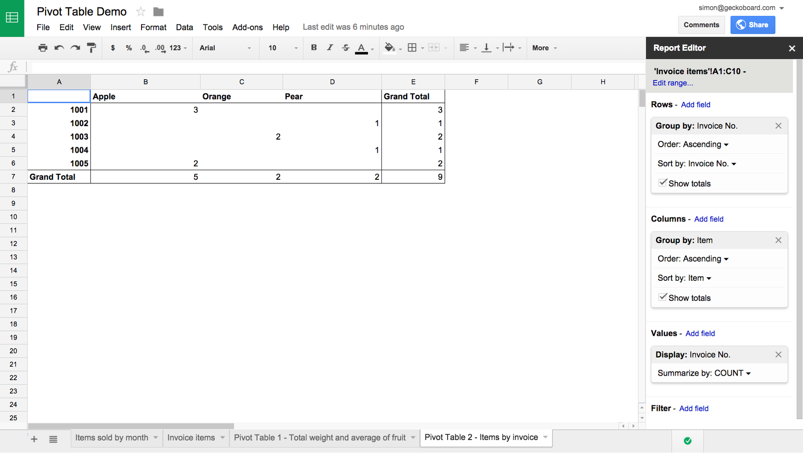
These examples just touch upon what you can do with pivot tables. You can find a lot more help for pivot tables in the Google Sheets support center.
If you get hooked on pivot tables the QUERY function is also well worth a look. It’s got a steeper learning curve (there’s no nice editor to play with) but it allows you to run some basic SQL-like queries.
The Coding Is For Losers blog has an excellent introduction to the QUERY function.
More useful articles on Google Sheets
Beyond Google Sheets: visualizing and sharing your data
Want to take your spreadsheet game even further? Now that you’ve imported data from various sources into your Google Sheets spreadsheets, you can easily visualize and share this information using a dashboard.
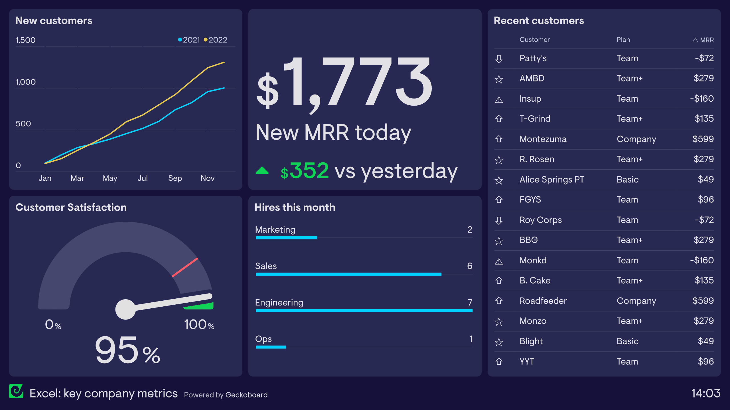
Learn more about this spreadsheet dashboard example here.
The example above contains a variety of visualizations, which can be powered either by Google Sheets or an Excel spreadsheet, which updates automatically to show up-to-the-minute data.
Here's how it works
- Create your spreadsheet in Google Sheets (importing data from via the steps mentioned earlier in this post)
- Sign up for a free Geckoboard account
- Select ‘Add dashboard’, then ‘Add widget’
- Pick the ‘Spreadsheet’ integration from the list of data sources.
- Select your data and choose a visualization
- Build out your dashboard by adding more visualizations
Watch this in action in the video below!
Originally published on 10th September 2015, updated on 5th October 2022
